The problem: anticipating rising water levels
The Vilaine, the main river in Brittany (France), flows through a watershed where winter floods are a recurring risk. In January 2025, a major flood once again highlighted the vulnerability of towns in the upper basin, from Vitré to Châteaubourg.
Traditional hydrological models (conceptual or physics-based) are valuable, but their implementation remains complex and their adaptation to real-time limited. The goal of this project: build an operational machine learning model capable of providing reliable predictions of water level (H) and flow rate (Q) across 11 stations simultaneously, with a horizon of 1 to 24 hours, and confidence intervals to quantify uncertainty.

The basin covers 4 rivers — the Vilaine (main axis), the Valière, the Cantache and the Veuvre/Chevré — with 3 dams whose releases directly influence downstream flood dynamics. The propagation time between the upstream end (Bourgon) and downstream (Cesson-Sévigné) is 11 to 27 hours depending on flow rate, which aligns well with our 24-hour prediction horizon.
The data: combining hydrology and weather
A good model starts with good data. I collected and combined two complementary sources, covering the period 2000 – 2026:
Hydrological data — Hydro EauFrance API
For each of the 11 stations in the basin (from upstream to downstream), I retrieved hourly time series of water level (H) and flow rate (Q) via the public Hydro EauFrance API. The API only returns one year of data per request: the collection script automatically splits the range into annual segments, handles retries, and operates incrementally — re-running the collection only fetches new data.
Weather data — Open-Meteo
For each station, I collected hourly precipitation (mm/h) and soil moisture (layers 0-7 cm and 7-28 cm) from the free Open-Meteo API. Soil moisture is a valuable indicator: already-saturated soil significantly amplifies runoff during a rainfall event.
Feature engineering
Raw data goes through a 7-step transformation pipeline to produce a training-ready dataset. Each station is characterized by 7 variables at each time step:
The derivative features (dH/dt and dQ/dt) capture the dynamics — is the level rising or falling, and how fast? For the 3 stations located downstream of dams, I added a "release" feature that detects water releases: a drop in water level without associated rainfall is a characteristic signal of a valve opening.
Normalization uses P1/P99 percentiles rather than min/max, making it robust to extreme values while preserving flood information.
Model architecture
The architecture I designed, called Station-Attention, combines three key ideas: treat each station as a distinct entity, let stations "talk to each other" via attention, and natively quantify uncertainty.
72h × 7 variables × 11 stations
24h forecasts per station
Each station encoded independently → 1 embedding / station
8 heads · Stations exchange spatial information
Water level
Flow rate
11 stations × 24 horizons × 3 quantiles (q10, q50, q90)
Why a shared LSTM?
A single LSTM network processes all 11 stations, forcing the model to learn generic hydrological patterns (flood rise, recession, rainfall response) rather than local peculiarities. Each station enters with its 7 variables and outputs an embedding vector that summarizes its recent dynamics.
Multi-station attention: the key component
It's the cross-attention layer (Multi-Head Attention, 3 layers × 8 heads) that gives the model its power. Concretely, it allows each station to consult the state of others to refine its own prediction. If an upstream station shows a rapid rise, downstream stations "know" a flood wave is approaching, even if nothing has happened locally yet. This mechanism naturally captures the spatial and temporal propagation of floods along the basin.
Quantile regression: measuring uncertainty
Rather than a single predicted value, the model provides three quantiles for each prediction: q10 (lower bound), q50 (median prediction), and q90 (upper bound). This gives an 80% confidence interval directly usable for risk management.
Prediction example with confidence intervals
Training: the details that matter
The model is implemented in PyTorch and trained on an NVIDIA DGX Spark equipped with a Blackwell GB10 GPU with 128 GB of unified memory — a welcome comfort for handling 25 years of data across 11 stations.
Asymmetric loss function
I use a pinball loss (the standard quantile regression loss) with a specific asymmetric penalty: during floods, underestimating the water level is far more dangerous than overestimating it. When the level at Châteaubourg exceeds 800 mm, the underestimation penalty is doubled. This is as much a domain decision as a technical one.
Flood oversampling
Floods are inherently rare events in the data. Without correction, the model would be excellent under normal conditions but mediocre during floods — precisely when accuracy matters most. I implemented progressive oversampling of flood periods in the training set:
Training strategy
Optimization uses AdamW with weight decay, a linear warmup over 5 epochs followed by a ReduceLROnPlateau scheduler. Gradients are clipped at 1.0 to stabilize training. Early stopping with a patience of 20 epochs on validation loss monitors overfitting.
The data split is strictly chronological to prevent information leakage: 25.5 years of training (2000 – June 2025), 6 months of validation (July – December 2025), and winter 2025-2026 for testing.
Results
The metrics below are measured on the test set (winter 2025-2026, data never seen during training), at the Châteaubourg station — the basin's reference station. The prediction is the median quantile (q50).
Real-time predictions — Châteaubourg, February 2026
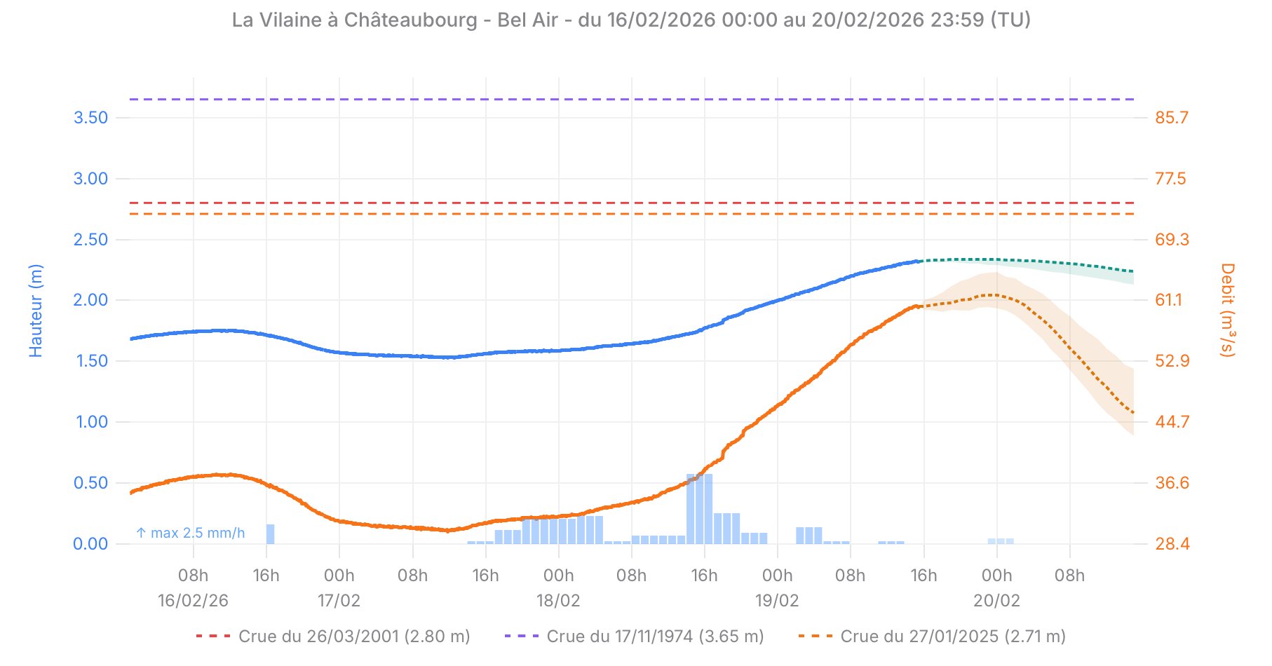
Water level (blue) and flow rate (orange) observed and predicted at Châteaubourg. The colored bands represent the confidence interval [q10 – q90]. The dashed lines indicate historical reference flood levels.
| Horizon | NSE | RMSE | Interpretation |
|---|---|---|---|
| t + 1h | 0.9999 | 6 mm | Near-perfect — the model has very strong natural inertia |
| t + 6h | 0.9967 | 36 mm | Excellent — well above the operational utility threshold |
| t + 12h | 0.9887 | 67 mm | Very good — uncertainty increases but remains controlled |
| t + 24h | 0.9710 | 108 mm | Good — an NSE > 0.97 at D+1 is a solid result |
NSE (Nash-Sutcliffe Efficiency) is the reference metric in hydrology. An NSE of 1 means a perfect prediction, an NSE of 0 means the model does no better than the historical mean. In practice, an NSE above 0.75 is considered "good" and above 0.90 "excellent". Our results are well beyond these thresholds, even at the 24-hour horizon.
Production deployment
A model that only runs in a notebook has limited value. The pipeline is designed end-to-end for real production deployment:
The PyTorch model is exported to ONNX format, a standard format that enables inference from any language. In this case, the model runs in a Node.js backend via onnxruntime-node, eliminating the Python dependency in production. Normalization parameters and metadata are also exported to ensure that inference preprocessing is identical to training.
Data collection runs continuously with the same scripts used for training — in incremental mode — ensuring consistency between training and production data.
Tech stack
What this project demonstrates
Beyond the numbers, this project illustrates a complete approach to applied machine learning — from raw data collection to production deployment. Designing a high-performing model also means building a robust pipeline, choosing an architecture suited to the business problem, and making the right engineering decisions (asymmetric loss, oversampling, ONNX export...).
This is exactly the type of engagement I deliver as a freelancer: turning a business problem into an operational, reliable, and maintainable machine learning system.
See the project: vilaine-amont.haruni.net · Source code on GitHub · Model on Hugging Face